9 VIsUaLiZe Data Relation with ggplot2

Size Venn Diagram xkcd 2122

We will use this iris dataset to demonstrate.

new_iris <- iris %>% 
            mutate(mutate_species= sample(Species),
                sepal_long= if_else( Sepal.Length >= median(Sepal.Length),1,0),
                petal_long= if_else( Petal.Length >= median(Petal.Width),1,0)) %>%
            dplyr::select(Species,mutate_species,sepal_long,petal_long)

new_iris %>% 
  head(10) %>% 
  knitr::kable() %>%
  kable_styling("striped", full_width = F) %>% 
  scroll_box(width = "500px", height = "200px")

Species	mutate_species	petal_long
setosa	versicolor	1
setosa	virginica	1
setosa	setosa	1
setosa	setosa	1
setosa	versicolor	1
setosa	setosa	1
setosa	setosa	1
setosa	versicolor	1
setosa	versicolor	1
setosa	versicolor	1

9.1 Venn diagram

9.1.1 ggVennDiagram

library(ggVennDiagram)

9.1.2 eulerr package

library(eulerr)

9.2 upset plot

library(UpSetR)

new_iris %>% 
  dplyr::select(-c(Species,mutate_species)) %>% 
  upset(.,empty.intersections = TRUE)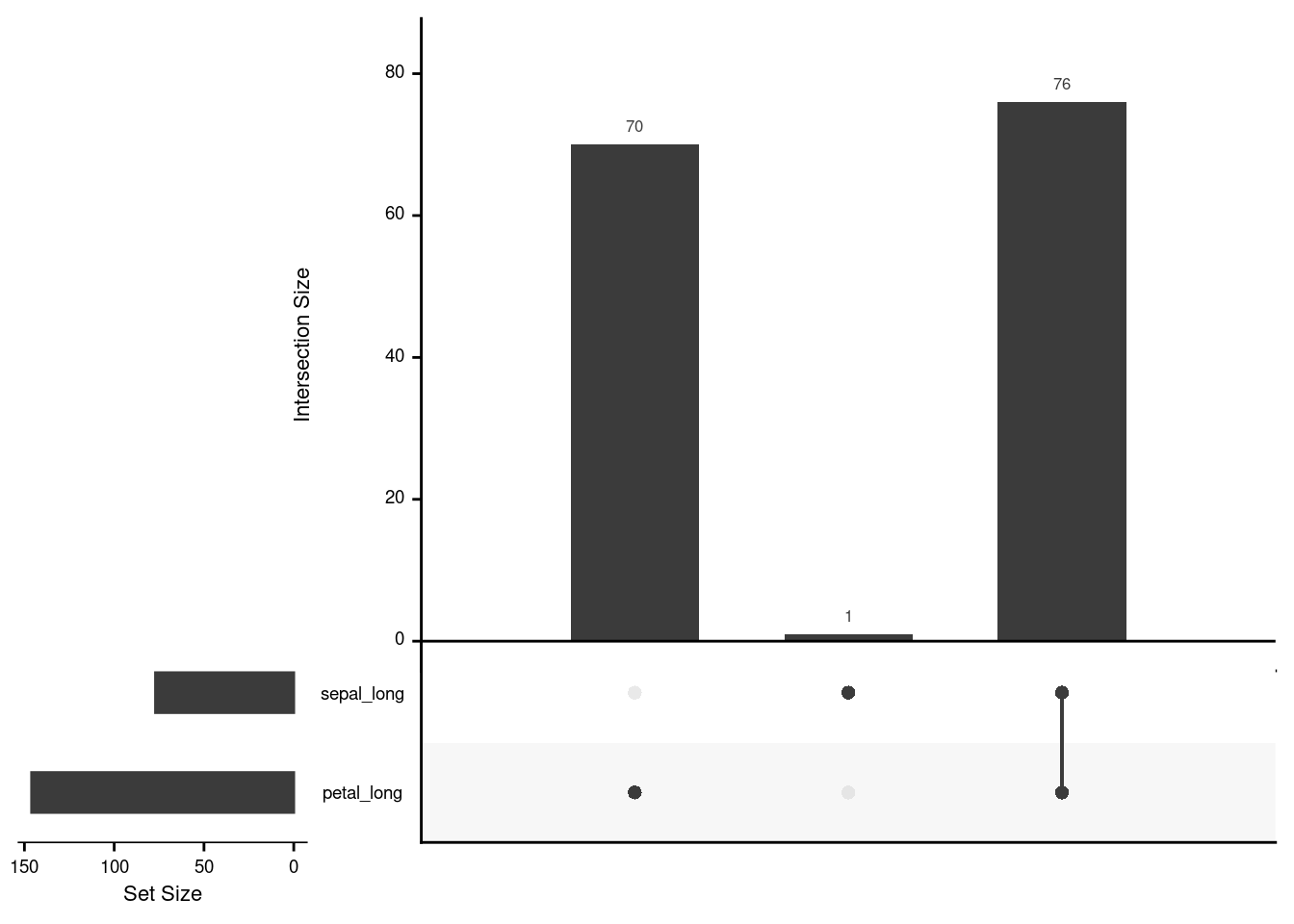

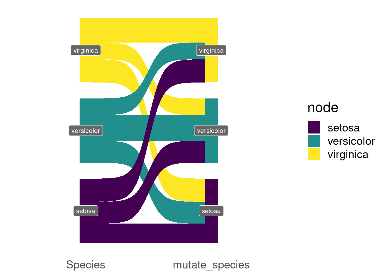
9.3 sankey plot with ggsankey

#install package with renv
renv::install("davidsjoberg/ggsankey")

#install package with devools
devtools::install_github("davidsjoberg/ggsankey")

library(ggsankey)

new_iris_sankey <- new_iris %>%
  make_long(Species,mutate_species)
  
  ggplot(new_iris_sankey ,aes(x = x, 
               next_x = next_x, 
               node = node, 
               next_node = next_node,
               fill = node,
               label= node)) +
  geom_sankey() +
  labs(x = NULL) +
  geom_sankey_label(size = 3, color = "white", fill = "gray40") +
  scale_fill_viridis_d() +
  theme_sankey(base_size = 18)